Layers
- Input
- Hidden
- Output
Multi Layers
- tf.keras.Sequential([layer1, layer2, layer3])
Output
- $y \in R^d$
- linear regression
- naive classification with MSE
- other general prediction
- out = relu(X@W + b)
- logits: 最后一层不加relu激活函数,输出叫做logits
- $y \in [0,1]$
- binary classification
- image generation
- rgb:将图片的数据归一化到[0,1]
- tf.sigmoid函数:只能保证单个点的值范围是[0,1],不能保证所有的输出值的和为1
- tf.softmax函数:用于多分类问题,保证每个值的范围为[0, 1],并且所有值的和为1
- tf.tanh:将值压缩到[-1,1]
Loss Function
MSE
- $MSE = \frac{1}{N}\sum(y-out)^2$
- $L2 = \sqrt{\sum(y-out)^2}$
- 两者可以转换 $MSE = norm(y-(x@w+b))^2$
import tensorflow as tf
import os

os.environ['TF_CPP_MIN_LOG_LEVEL'] = '2'
y = tf.constant([1, 2, 3, 0, 2])
y = tf.one_hot(y, depth=4)
y = tf.cast(y, dtype=tf.float32)
out = tf.random.normal([5, 4])

loss1 = tf.reduce_mean(tf.square(y - out))
loss2 = tf.square(tf.norm(y - out)) / (5 * 4)
loss3 = tf.reduce_mean(tf.losses.MSE(y, out))
print(f'loss1: {loss1}, loss2: {loss2}, loss3: {loss3}')  # MSE is a function, MeanSquareError is a class
Cross Entropy Loss
Entropy
熵是用来衡量不确定性的,熵越低,越稳定,分布均匀,熵越大,不稳定,分布越不均匀
- uncertainty
- measure of surprise
- lower entropy -> more info -> more stable
$$ H(p) = - \sum_{i} P(i)\log P(i) $$
注意是以2为底计算,但是tf是使用e为底计算的,所以需要除以loge(2)
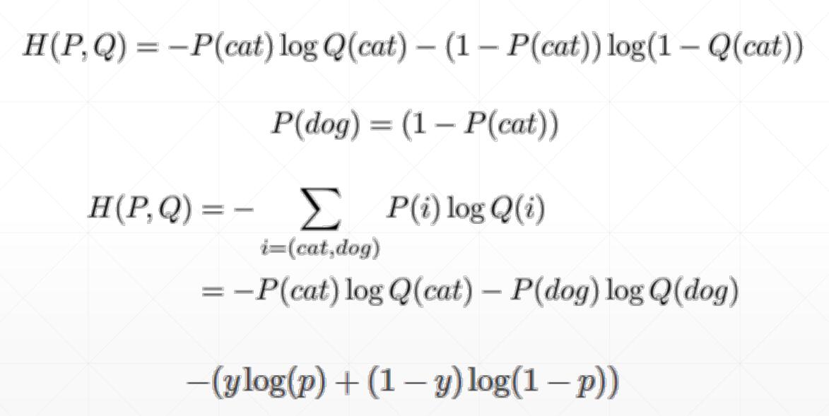
Cross Entropy
交叉熵是用来衡量两个分布之间的信息的衡量标准
$$ H(p,q) = -\sum p(x) \log q(x) = H(p) + D{KL} (p|q) $$
for p = q, minima: $H(p,q)=H(p)$
在多分类问题中,我们经常使用one-hot编码标签p,有:
- $h(p:[0,1,0]) = -0log0 -1log1 - 0log0 = 0$
- $H([0,1,0], [q1,q2,q3]) = H(p) + D_{KL}(p|q) = 0 + (-1\log q_i) = 0$
Binary Classification
Single output:
Why not MSE
- sigmoid + MSE
- gradient vanish
- converge slower
但是在meta-learning中,MSE效果较好
Logits -> Cross Entropy
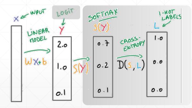
因为在计算交叉熵的时候,自己写的代码从进行softmax操作出现除以0的数值不稳定情况,因此最好不要做softmax操作,而是选择直接使用tf提供的封装函数。
import tensorflow as tf
print('Numerical Stability')
x = tf.random.normal([1, 784])
w = tf.random.normal([784, 2])
b = tf.zeros([2])

logits = x @ w + b
print(logits)

prob = tf.math.softmax(logits, axis=1)
print(prob)

print(tf.losses.categorical_crossentropy([0, 1], logits, from_logits=True))  # 非常重要,默认是False
print(tf.losses.categorical_crossentropy([0, 1], prob))
在tf.keras中,有两个交叉熵相关的损失函数tf.keras.losses.categorical_crossentropy和tf.keras.losses.sparse_categorical_crossentropy。其中sparse的含义是,真实的标签值y_true可以直接传入int类型的标签类别。具体而言:
loss = tf.keras.losses.sparse_categorical_crossentropy(y_true=y, y_pred=y_pred)
与
loss = tf.keras.losses.categorical_crossentropy(
    y_true=tf.one_hot(y, depth=tf.shape(y_pred)[-1]),
    y_pred=y_pred
)
的结果相同。
AutoGrad
详见Code
- with tf.GradientTape() as tape: 默认情况下离开该上下文管理器,tape就会被自动释放掉,要想多次调用就需要设置persistent=True
- build computation graph
- $loss = f_\theta (x)$
- [w_grad] = tape.gradient(loss, [w])
二阶求导:
import tensorflow as tf
# 二阶求导,基本上用不到
with tf.GradientTape() as t1:
    t1.watch([w, b])  # 很重要,跟踪梯度信息
    with tf.GradientTape() as t2:
        t2.watch([w, b]) # 很重要,跟踪梯度信息
        y4 = x * w ** 2 + 2*b
        dy_dw, dy_db = t2.gradient(y4, [w, b])
d2y_dw2 = t1.gradient(dy_dw, w)
print(dy_dw, dy_db)
print(d2y_dw2)
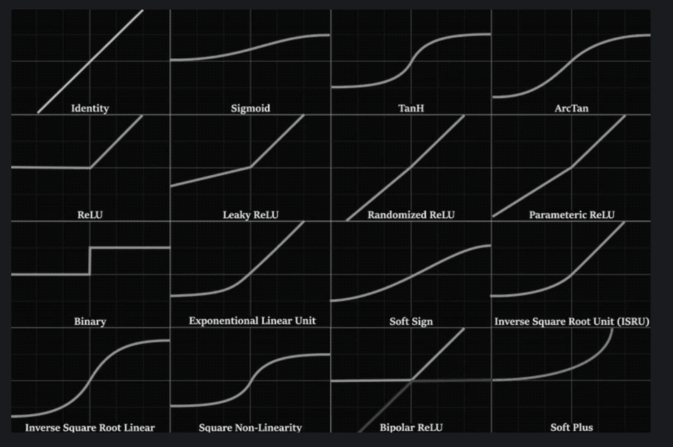
Activation Function and Gradients
- sigmoid
- tanh
- relu
Reference
Note: Cover Picture