Super Agents of AI

Terminology & Notation

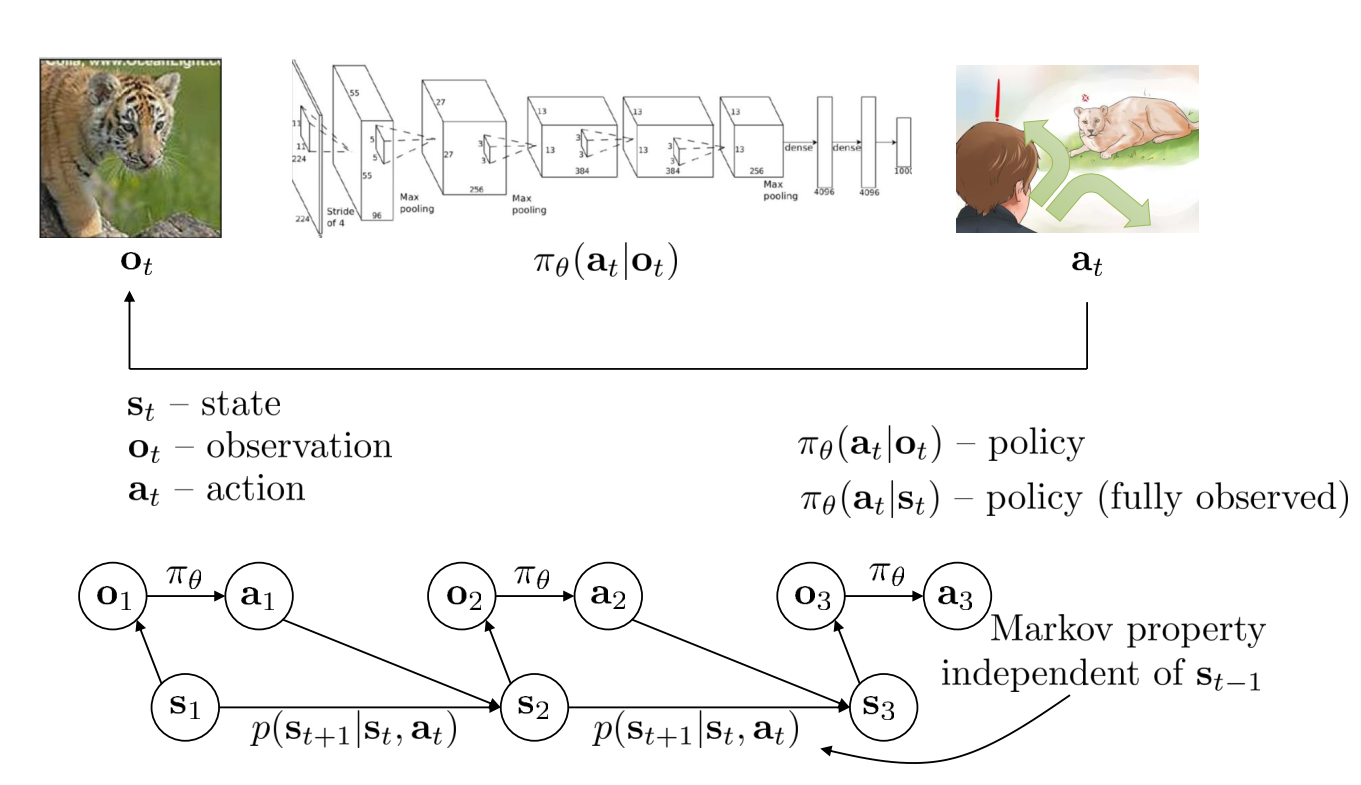
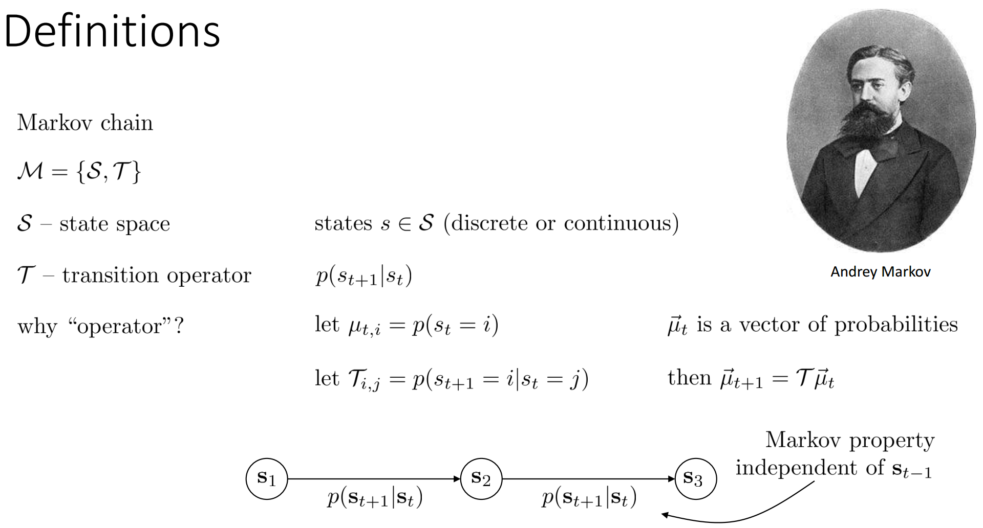
Definitions

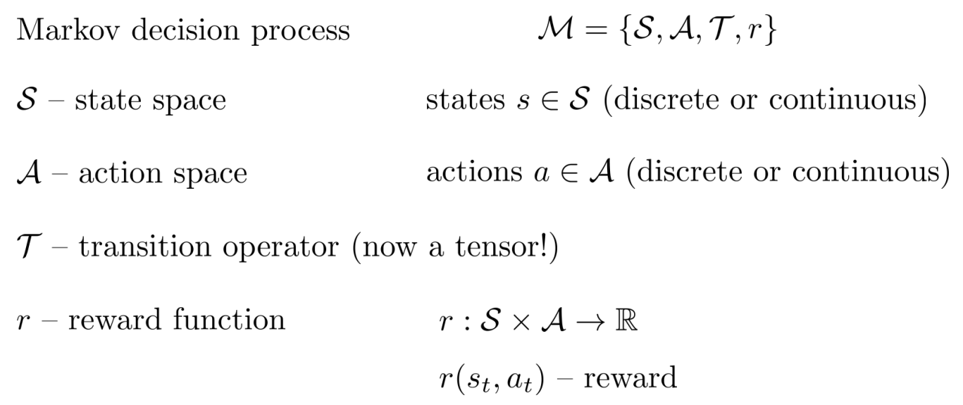
MDP

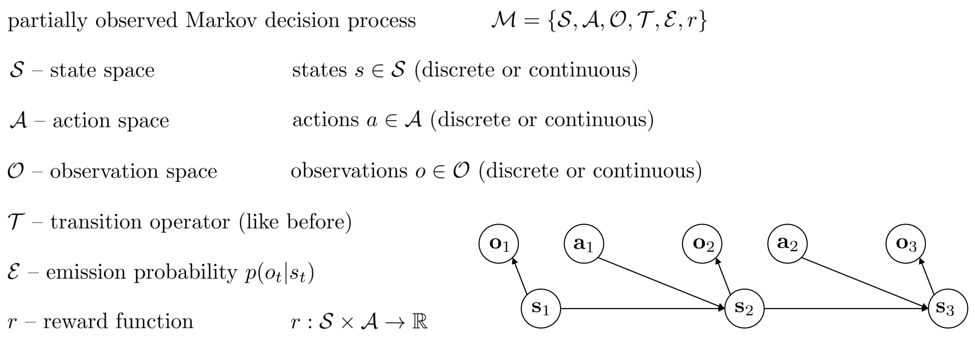
POMDP

The Goal of Reinforcement Learning

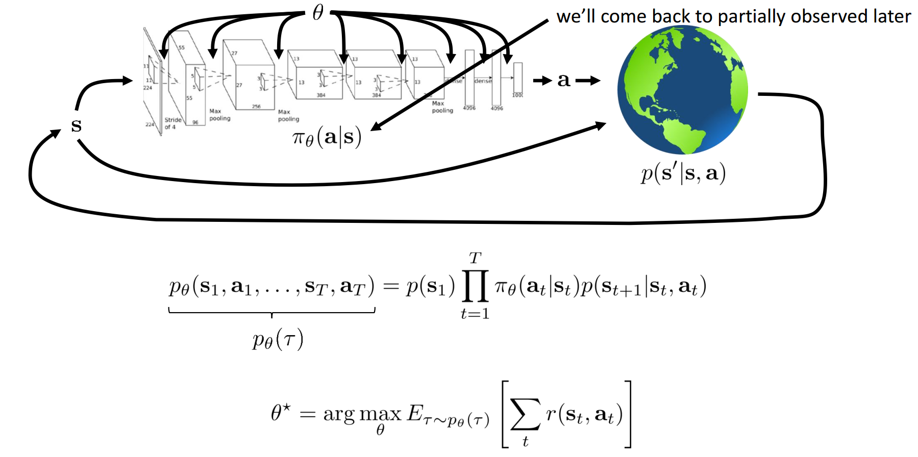
Markov chain on $(s,a)$:

$p((s_{t+1}, a_{t+1})| (s_t, a_t)) = p(s_{t+1}|s_t, a_t) \pi_\theta(a_{t+1}|s_{t+1})$

Finite Horizon Case: State-action Marginal

$p_\theta(s_t,a_t)$ is state-action marginal.

$\theta^* = arg \max_{\theta} E_{\tau \sim p_\theta(\tau)} \left [ \sum_t r(s_t, a_t) \right ] = arg \max_{\theta} \sum_{t=1}^T E_{(s_t,a_t) \sim p_{\theta}(s_t,a_t) } \left [ r(s_t, a_t) \right ]$

Infinite Horizon Case: Stationary Distribution

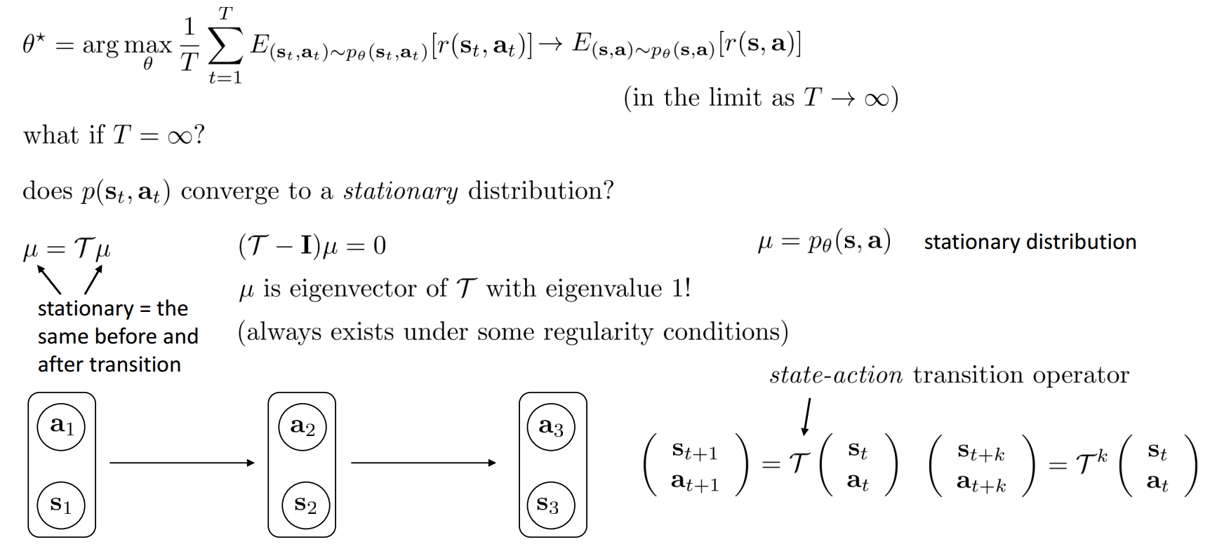
Expectations and Stochastic Systems

For infinite horizon case:

$\theta^* = arg \max_\theta E_{(s,a) \sim p_\theta(s,a)} \left [r(s,a) \right]$

For finite horizon case:

$\theta^* = arg \max_\theta \sum_{t=1}^T E_{(s_t,a_t) \sim p_\theta(s_t,a_t)} \left [r(s_t,a_t) \right ]$

In RL, we almost always care about expectations.

• $r(x)$ -> not smooth
• $\pi_\theta(a=fall) = \theta$
• $E_{\pi_\theta}\left [ r(x) \right]$ -> smooth in $\theta$!

RL Algorithms

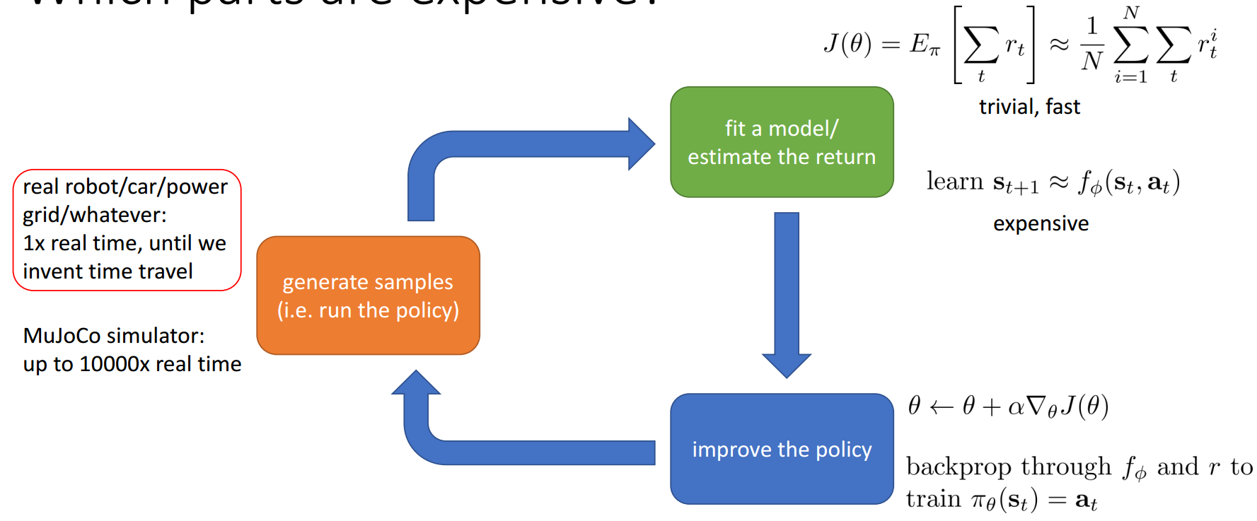
Structure of RL Algorithms

• Sample generation
• Fitting a model/estimating return
• Policy improvement

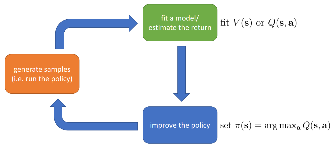
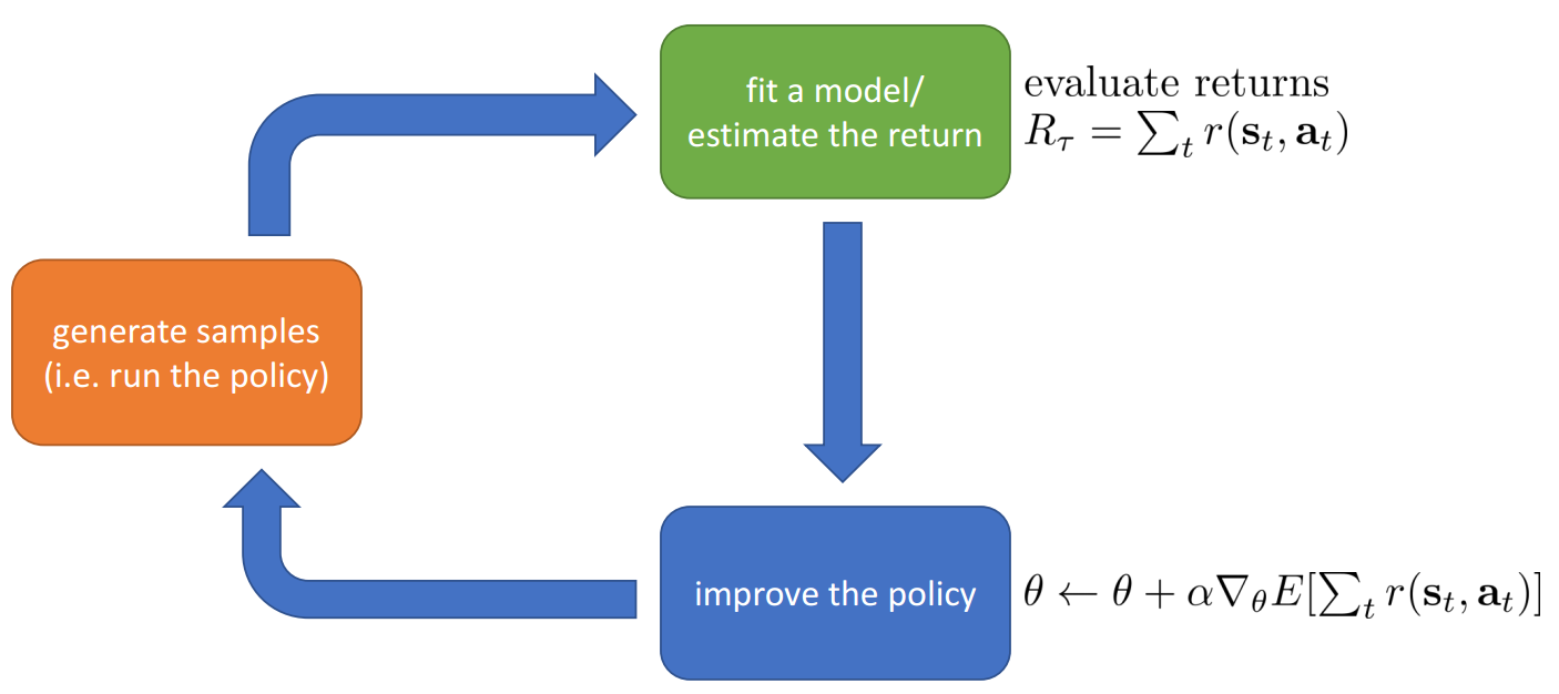
The Anatomy of a RL Algorithm

Q-Function

Q-function is the total reward from taking $a_t$ in $s_t$:

$Q^{\pi}(s_t,a_t) = \sum_{t\prime = t}^T E_{\pi_\theta} \left[ r( s_t\prime, a_t\prime ) | s_t, a_t \right ]$

Value-Function

Value-function is the total reward from $s_t$:

$V^\pi(s_t) = \sum_{t\prime = t}^T E_{\pi_\theta} \left [ r(s_{t\prime},a_{t\prime} ) | s_t \right ]$

$V^\pi(s_t) = E_{a_t \sim \pi(a_t|s_t)} \left [ Q^\pi(s_t, a_t) \right ]$

$E_{s_1 \sim p(s_1)} \left [ V^\pi(s_t) \right ]$ is the RL objective!

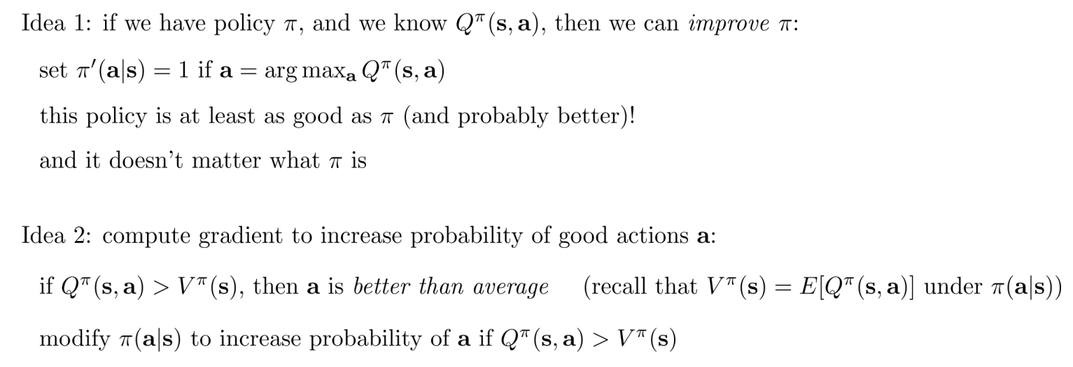
Using Q-Function and Valuer Functions

Types fo RL Algorithms

The goal of RL:

$\theta^* = arg \max_{\theta} E_{\tau \sim p_\theta(\tau)} \left [ \sum_t r(s_t, a_t) \right ]$

• Policy gradients: directly differentiate the above objective
• Value-based: estimate value function or Q-function of the optimal policy (no explicit policy)
• Actor-critic: estimate value function or Q-function of the current policy, use it to improve policy
• Model-based RL: estimate the transition model, then improve the policy

Model-based RL

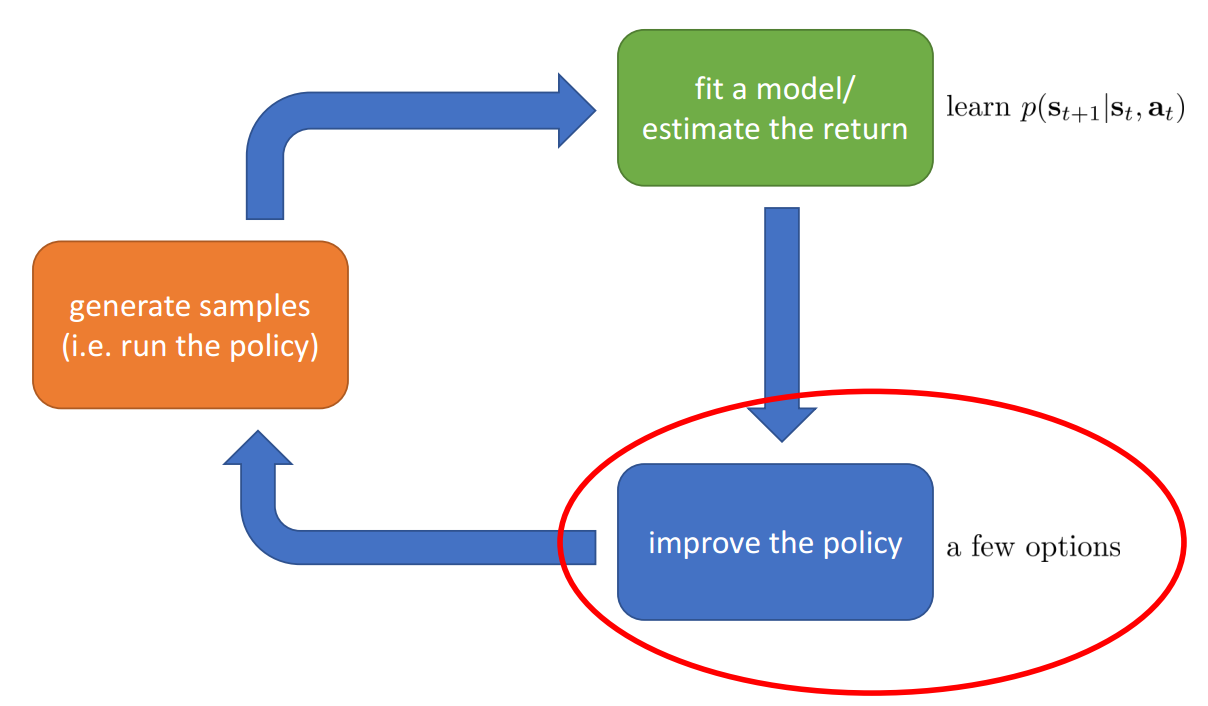
Estimate the transition model, then improve the policy by:

• Just use the model to plan (no policy)
  • Trajectory optimization/optimal control (primarily in continuous spaces) – essentially back-propagation to optimize over actions
  • Discrete planning in discrete action spaces – e.g., Monte Carlo tree search
• Back-propagate gradients into the policy
  • Requires some tricks to make it work
• Use the model to learn a value function
  • Dynamic programming
  • Generate simulated experience for model-free learner

Value-Function based RL

Direct Policy Gradients

Actor-Critic: Value Functions + Policy Gradients

Why So Many RL Algorithms

• Different tradeoffs
  • Sample efficiency
  • Stability & ease of use
• Different assumptions
  • Stochastic or deterministic?
  • Continuous or discrete?
  • Episodic or infinite horizon?
• Different things are easy or hard in different settings
  • Easier to represent the policy?
  • Easier to represent the model?

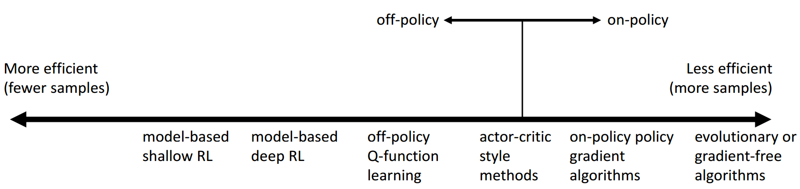
Comparison: Sample Efficiency

Sample efficiency: how many samples do we need to get a good policy?

Most important question: is the algorithm off policy?

• Off policy: able to improve the policy without generating new samples from that policy
• On policy: each time the policy is changed, even a little bit, we need to generate new samples

Comparison: Stability and Ease of Use

Question:

• Does it converge?
• And if it converges, to what?

• And does it converge every time?

• Supervised learning: almost always gradient descent

• Reinforcement learning: often not gradient descent

  • Q-learning: fixed point iteration
    • At best, minimizes error of fit (“Bellman error”)
      • Not the same as expected reward
    • At worst, doesn’t optimize anything
      • Many popular deep RL value fitting algorithms are not guaranteed to converge to anything in the nonlinear case
  • Model-based RL: model is not optimized for expected reward
  • Model minimizes error of fit
    • This will converge
    • No guarantee that better model = better policy
  • Policy gradient
    • The only one that actually performs gradient descent(ascent) on the true objective, but also often the least efficient!

Comparison: Assumptions

• Common assumption #1: full observability
  • Generally assumed by value function fitting methods
  • Can be mitigated by adding recurrence
• Common assumption #2: episodic learning
  • Often assumed by pure policy gradient methods
  • Assumed by some model-based RL methods
• Common assumption #3: continuity or smoothness
  • Assumed by some continuous value function learning methods
  • Often assumed by some model-based RL methods

Examples of Specific Algorithms

• Value function fitting methods
  • Q-learning, DQN
  • Temporal difference learning
  • Fitted value iteration
• Policy gradient methods
  • REINFORCE
  • Natural policy gradient
  • Trust region policy optimization
• Actor-critic algorithms
  • Asynchronous advantage actor-critic (A3C)
  • Soft actor-critic (SAC)
• Model-based RL algorithms
  • Dyna
  • Guided policy search

Note: Cover Picture