Super Agents of AI

Matrix Factorization

The user-item, or ratings matrix is N * M, where N is the number of users and M is the number of items.

Rethink about R

• Key: W and U should be much smaller than R
• Actually, we can’t stored R in our memory since it too large.
• But we can represent it using a special data structure: Dict{(u,m) -> r}
• If N = 120K, M = 26K
  • N * M = 3.38 billion
  • # ratings = 20 million
  • Space used: 20 million / 3.38 billion = 0.006
• This is called a “Sparse representation”

Matrix Factorization

Matrix factorization is to split the matrix into the product of 2 other matrix.

We call it “R hat” because it only approximates R - it is our model of R. The formula is shown below:

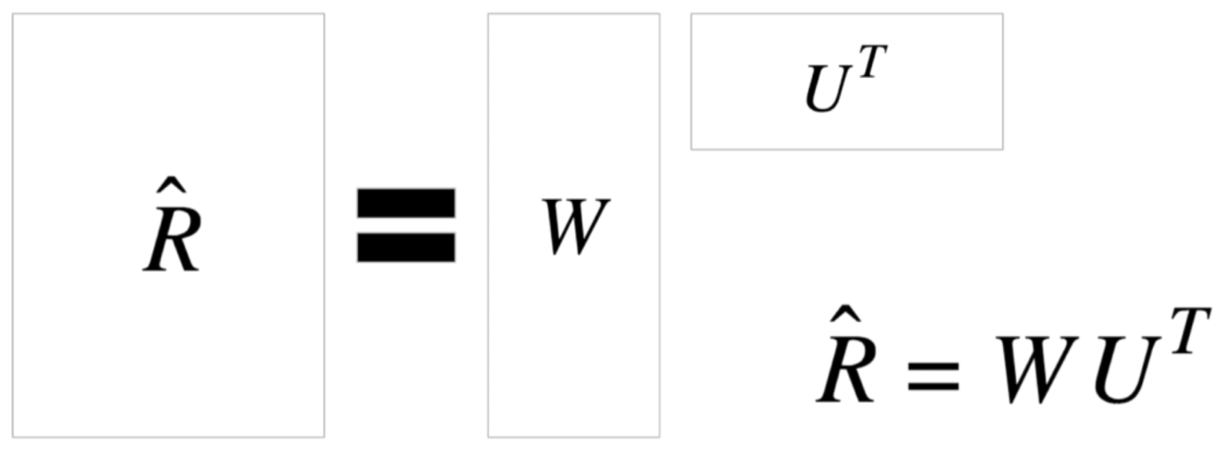
So we would like W and U to be very skinny:

• W (N * K)： the users matrix
• U (M*K)：the movies matrix
• K：somewhere from 10-50

Some Calculations

if K = 10, N = 130K, M = 26K, then:

• W: 130K * 10 = 1.3 million
• U: 26K * 10 = 0.26 million
• Total size of W + U = 1.3 million + 0.26 million = 1.56 million
• How much saving: 1.56 million / 3.38 billion = 0.0005

This is good, we like # parameters < # of data points.

In practice, we don’t calculate the WU^T which makes the result R (N * M) unless in a small subset of data.

Actually, we often calculate one rating like the score of user i rating item j. It just a dot product between 2 vectors of size K:

$\hat{r_{ij}} = w_i^T u_j, \hat{r_{ij}} = \hat{R[i,j]}, w_i = W[i], u_j = U[j]$

Why does it make sense

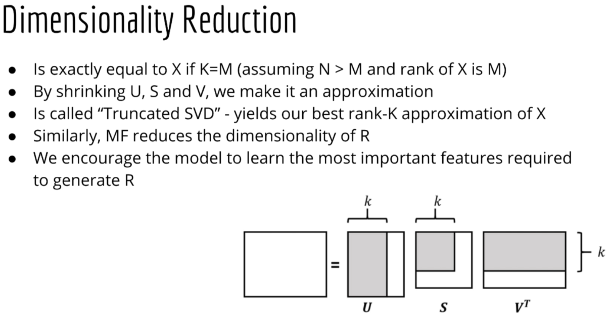
Singular Value Decomposition also known as SVD is a matrix X can be decomposed into 3 separate matrices multiplied together:

$X = USV^T$

Where:

• X (N * M), U (N * K), S (K * K), V (M * K)
• If I multiply U by S, I just get another N * K matrix:
  • Then X is a product of 2 matrices, just like matrix factorization
  • Or equivalently, I could combine S with V^T
• R (ratings matrix) is sparse
  • If U, S, and V can properly approximate a full X matrix, then surely it can approximate a mostly empty R matrix!
    

Interpretation

• Each of the K elements in w_i and u_j is a feature
• Let’s suppose K = 5, and they are:
  • Action / adventure
  • Comedy
  • Romance
  • Horror
  • Animation
• w_i[1] is how much user i likes action
• w_i[2] is how much user i likes comedy, etc
• u_j[1] is how much movie_j contains action
• u_j[2] is how much movie_j contains comedy, etc

The w_i^Tu_j means how well do user i’s preferences correlate with movie j’s attributes:

$w_i^Tu_j = || w_i || ||u_j|| \cos{\theta} \propto sim(i,j)$

Actually, each features is latent, and K is the latent dimensionality, a.K.A “Hidden causes”. We don’t know the meaning of any feature without inspecting it.

Dimensionality Reduction

MF reduces the dimensionality of R.

How to Learn W nad U

Loss Function

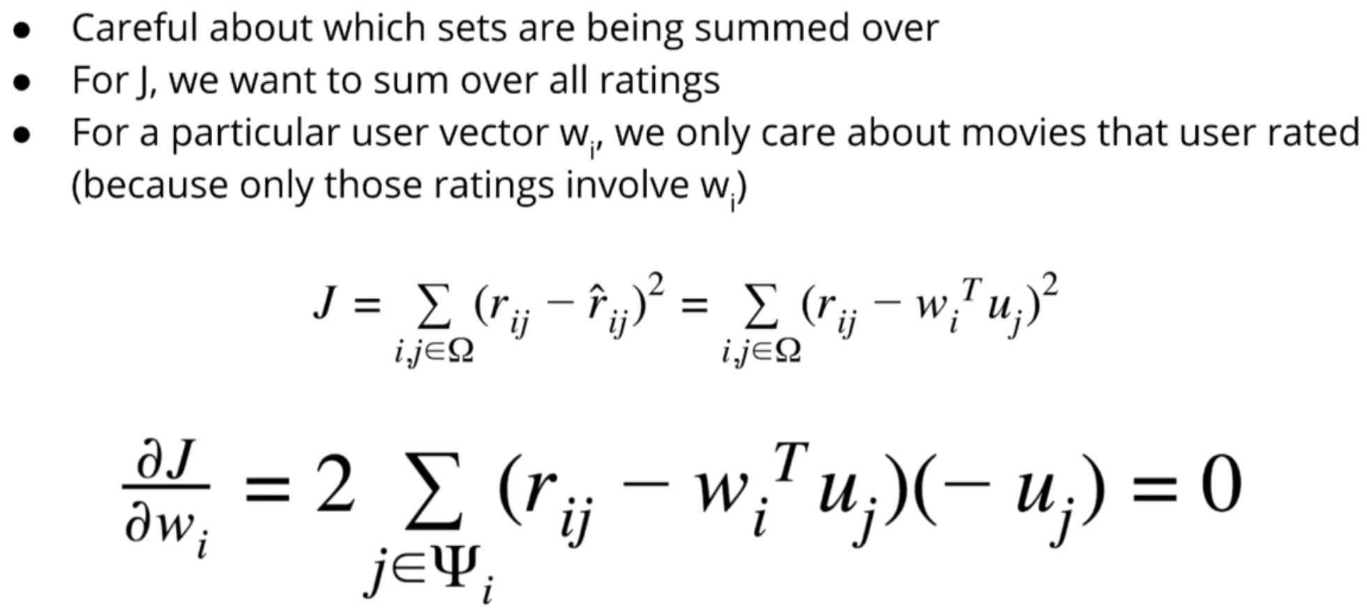
Using the squared error loss as the loss function:

$J = \sum_{i,j \in \omega} (r_{ij} - \hat{r}_{ij})^2 = \sum_{i,j \in \omega} (r_{ij} - w_i^T u_j)^2$

Omega = set of pairs (i,j) where user i rated movie j.

Solving for W

Try to isolate w_i, it’s stuck inside a dot product:

$\sum_{j \in \Psi} (w_i^T u_j) u_j = \sum_{j \in \Psi} r_{ij} u_j$

Dot product is commutative:

$\sum_{j \in \Psi} (u_j^T w_i) u_j = \sum_{j \in \Psi} r_{ij} u_j$

The result of dot product is a scalar, so scalar * vector = vector * scalar:

$\sum_{j \in \Psi} u_j (u_j^T w_i) = \sum_{j \in \Psi} r_{ij} u_j$

Drop the brackets:

$\sum_{j \in \Psi} u_j u_j^T w_i = \sum_{j \in \Psi} r_{ij} u_j$

Summation doesn’t actually depend on i, so add more brackets:

$\sum_{j \in \Psi} (u_j u_j^T) w_i = \sum_{j \in \Psi} r_{ij} u_j$

Now it’s just Ax=b, which we know how to solve:

x = np.linalg.solve(A, b)

$w_i = (\sum_{j \in \Psi} u_j u_j^T)^{-1} \sum_{j \in \Psi} r_{ij} u_j$

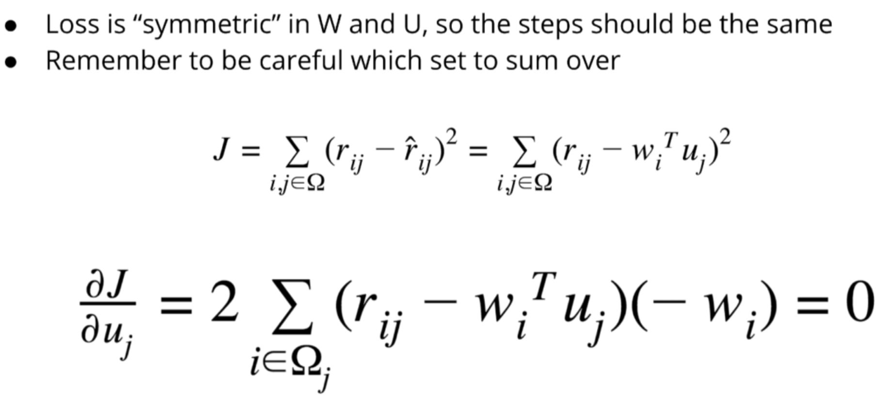
Solving for U

Note: Cover Picture