Rainbow
Rainbow算法主要有七个核心知识点组成:
- Deep Q Learning Network (DQN)
- Double Q Learning Network (DDQN)
- Prioritized Experience Replay (PER)
- Dueling Network
- Noisy Networks for Exploration
- Categorical DQN
- N-Step Learning
Deep Q Learning Network (DQN)
强化学习算法的目标是根据当前的状态,选择能够使累计奖惩值最大的动作值给智能体执行。当使用非线性函数逼近器如神经网络拟合Q函数时,智能体的训练会产生不稳定甚至发散的情况,主要原因在于:
- 观察序列中存在相关性
- 对当前Q的小步更新都可能显著影响策略,而今使更新后的策略采集的数据分布和更新前的不一致,进而改变Q值与目标值之间的相关性
在DQN中,作者提出两个解决方法:
- Replay Buffer:强化学习训练时会将智能体的经验根据时间顺序连续保存到经验回放池中(s, a, r, s’),会造成相邻两个样本之间存在相关性,解决思路是利用随机均匀采样经验池的中样本数据供智能体训练
- Fixed Q-Target:DQN使用定期迭代更新的方式更新目标值计算中的拟合网络参数,从而减少了与目标值之间的相关性,如果一直更新,会由于目标值一直改变不”稳定”而造成训练发散
DQN迭代更新的损失函数为:
$$ Loss_i(\theta_i) = \mathbb{E}_{(s,a,r,s\prime) \sim U(D)} \big[ \big( r + \gamma \max_{a\prime} Q(s\prime,a\prime;\theta_i^-) - Q(s, a; \theta_i) \big)^2 \big] $$
- 其中γ是折扣因子,用来决定目标值对于当前值的影响程度
- $\theta_i$代表第i次迭代过程的神经网络参数
- $\theta_(i-1)$代表目标值函数的神经网络参数
- 目标值函数的网络参数是每隔C次训练才更新,C次训练期间保持目标值函数的网络参数固定不变
为了增加训练的稳定性,作者还提出了梯度裁剪(Gradient Clipping)的方法,将$\big( r + \gamma \max_{a\prime} Q(s\prime,a\prime;\theta_i^-) - Q(s, a; \theta_i) \big)$差值限定在了[-1,1]之间。
代码实现细节技巧
通常Python实现经验回放池会用到三种数据结构:
- collections.deque: 底层实现是使用的双向链表,插入时间复杂度是O(1),但是查询的时间复杂度是O(n),会严重增加训练过程的时间
- list:列表底层是数组,存储的是指向不同或者相同大小物体的指针,可以动态增加数据和支持随机访问,比使用deque队列的方式要快
- numpy.ndarray:访问最快的数据结构,底层是存储的具有相同固定大小的同质数据,可以根据内存的访问局部性原理加快读取速度
ReplayBuffer参考实现:OpenAI spinning-up
class ReplayBuffer:
    """A simple FIFO numpy replay buffer."""

    def __init__(self, obs_dim: int, size: int, batch_size: int = 32):
        self.obs_buf = np.zeros([size, obs_dim], dtype=np.float32)
        self.next_obs_buf = np.zeros([size, obs_dim], dtype=np.float32)
        self.acts_buf = np.zeros([size], dtype=np.float32)
        self.rews_buf = np.zeros([size], dtype=np.float32)
        self.done_buf = np.zeros(size, dtype=np.float32)
        self.max_size, self.batch_size = size, batch_size
        self.ptr, self.size, = 0, 0

    def store(
            self,
            obs: np.ndarray,
            act: np.ndarray,
            rew: float,
            next_obs: np.ndarray,
            done: bool,
    ):
        self.obs_buf[self.ptr] = obs
        self.next_obs_buf[self.ptr] = next_obs
        self.acts_buf[self.ptr] = act
        self.rews_buf[self.ptr] = rew
        self.done_buf[self.ptr] = done
        self.ptr = (self.ptr + 1) % self.max_size
        self.size = min(self.size + 1, self.max_size)

    def sample_batch(self) -> Dict[str, np.ndarray]:
        idxs = np.random.choice(self.size, size=self.batch_size, replace=False)
        return dict(obs=self.obs_buf[idxs],
                    next_obs=self.next_obs_buf[idxs],
                    acts=self.acts_buf[idxs],
                    rews=self.rews_buf[idxs],
                    done=self.done_buf[idxs])

    def __len__(self) -> int:
        return self.size
Double DQN
在标准Q-learning和DQN算法中,取最大值的操作都是使用相同的Q值去选择和评估动作的好坏,这样会让智能体更加喜欢选择被过度估计的值,导致最终的价值估计过于乐观。
$$ \theta_{t+1} = \theta_t + \alpha \big(Y_t^Q - Q(S_t, A_t; \theta_t)\big) \cdot \nabla_{\theta_t} Q(S_t, A_t; \theta_t) $$
where $\alpha$ is a scalar step size and the target $Y_t^Q$ is defined as:
$$ Y_t^Q = R_{t+1} + \gamma \max_a Q(S_{t+1}, a; \theta_t) $$
在DDQN中,通过对两个不同的值函数随机采样经验样本训练并更新其中一个值函数的方式,学习到两套参数集合。$\theta$和$\theta\prime$。在每一次更新的过程中,其中一套参数被用来作为Greedy策略,另一套参数被选择用来决定它的值。
DQN的目标函数:
$$ Y_t^Q = R_{t+1} + \gamma \max_a Q(S_{t+1}, \arg\max_a Q(S_{t+1}, a; \theta_t); \theta_t). $$
DDQN的目标函数为:
$$ Y_t^{DoubleQ} = R_{t+1} + \gamma \max_a Q(S_{t+1}, \arg\max_a Q(S_{t+1}, a; \theta_t); \theta_t\prime). $$
代码实现细节
DQN
# G_t   = r + gamma * v(s_{t+1})  if state != Terminal
#       = r                       otherwise
curr_q_value = self.dqn(state).gather(1, action)
next_q_value = self.dqn_target(next_state).max(
    dim=1, keepdim=True)[0].detach()
mask = 1 - done
target = (reward + self.gamma * next_q_value * mask).to(self.device)

# calculate dqn loss
loss = F.smooth_l1_loss(curr_q_value, target)
DDQN
selected_action = dqn(next_state).argmax(dim=1, keepdim=True)
# gather的作用是只选择selected_action对应index的Q值
# Double DQN
next_q_value = self.dqn_target(next_state).gather(1, self.dqn(next_state).argmax(dim=1, keepdim=True)).detach()
mask = 1 - done
target = (reward + self.gamma * next_q_value * mask).to(self.device)

# calculate dqn loss
loss = F.smooth_l1_loss(curr_q_value, target)
Prioritized Experience Replay (PER)
使用经验回放池需要解决两个问题:
- 存储哪些动作序列
- 采样哪些动作序列
PER要解决的是第二个问题,即如何最有效地选择经验回放池中的样本数据进行学习,其核心思想是衡量每个动作序列样本的重要性程度。一种可行的方法是利用样本的TD-error来表示,因为这表明了这次样本的“惊喜”大小。该算法会存储经验回放池中每个样本的最后的TD-error值,然后根据最大绝对TD-error进行采样。Q-learning会利用采样到的样本进行训练和根据TD-error更新权重。当新的转换无法计算TD-error时,会将其误差设置为最大,从而保证所有的样本至少被采样一次。
计算TD-error的方式:
- Greedy TD-Error Prioritization: 最大的缺点是会聚焦于一小部分经验子集,当使用函数逼近的方法时,误差减小的慢,意味着一开始高误差的样本会被频繁重复地采样,这样的欠多样性样本使得训练的智能体很容易就过拟合
- Stochastic Prioritization:介于纯Greedy Prioritization和均匀随机采样之间:
$$ P(i) = \frac{p_i^{\alpha}}{\sum_k p_k^{\alpha}} $$
$p_i$代表样本i的优先级大小,指数$\alpha$代表使用优先级的影响程度,当$\alpha$为0时,代表均匀随机采样。在实际中,会添加一个正整数偏置常量$\epsilon$,$p_i=|\sigma_i| + \epsilon$,保证可以对所有的样本进行采样。
根据样本优先级采样的方式会带来偏差,因为其并不是均匀随机采样样本而是根据TD-error作为采样比例。为了修正该误差,作者引入了重要性采样(Importance-sampling, IS)权重:
$$ w_i = \big( \frac{1}{N} \cdot \frac{1}{P(i)} \big)^\beta $$
当$\beta = 1$,上面的式子完全补偿非均匀概率$𝑃_(𝑖)$,是的其最终为均匀概率。 通过使用$𝑤_𝑖\sigma_𝑖$而不是$\sigma_i$,可以将这些权重嵌入到Q-learning的更新中。
在典型的强化学习场景中,更新的无偏性质在训练结束时接近收敛是最重要的,因此,我们利用随着时间衰减重要性采样校正量来达到当训练结束,指数$\beta=1$,从而满足无偏条件。
代码实现细节
PrioritizedReplayBuffer的实现利用了Segment Tree数据结构,它在保存经验样本和采样样本的同时也负责管理样本的Priorities,是非常高效的实现方式。
class PrioritizedReplayBuffer(ReplayBuffer):
    """Prioritized Replay buffer.

    Attributes:
        max_priority (float): max priority
        tree_ptr (int): next index of tree
        alpha (float): alpha parameter for prioritized replay buffer
        sum_tree (SumSegmentTree): sum tree for prior
        min_tree (MinSegmentTree): min tree for min prior to get max weight

    """
    def __init__(self,
                 obs_dim: int,
                 size: int,
                 batch_size: int = 32,
                 alpha: float = 0.6):
        """Initialization."""
        assert alpha >= 0

        super(PrioritizedReplayBuffer, self).__init__(obs_dim, size,
                                                      batch_size)
        self.max_priority, self.tree_ptr = 1.0, 0
        self.alpha = alpha

        # capacity must be positive and a power of 2.
        tree_capacity = 1
        while tree_capacity < self.max_size:
            tree_capacity *= 2

        self.sum_tree = SumSegmentTree(tree_capacity)
        self.min_tree = MinSegmentTree(tree_capacity)

    def store(self, obs: np.ndarray, act: int, rew: float,
              next_obs: np.ndarray, done: bool):
        """Store experience and priority"""
        super().store(obs, act, rew, next_obs, done)
        # 这里保存的是默认值,还没有直接计算出来TD-Error
        self.sum_tree[self.tree_ptr] = self.max_priority**self.alpha
        self.min_tree[self.tree_ptr] = self.max_priority**self.alpha
        self.tree_ptr = (self.tree_ptr + 1) % self.max_size

    def sample_batch(self, beta: float = 0.4) -> Dict[str, np.ndarray]:
        """Sample a batch of experiences."""
        assert len(self) >= self.batch_size
        assert beta > 0

        indices = self._sample_proportional()

        obs = self.obs_buf[indices]
        next_obs = self.next_obs_buf[indices]
        acts = self.acts_buf[indices]
        rews = self.rews_buf[indices]
        done = self.done_buf[indices]
        weights = np.array([self._calculate_weight(i, beta) for i in indices])

        return dict(
            obs=obs,
            next_obs=next_obs,
            acts=acts,
            rews=rews,
            done=done,
            weights=weights,
            indices=indices,
        )

    def update_priorities(self, indices: List[int], priorities: np.ndarray):
        """Update priorities of sampled transitions."""
        assert len(indices) == len(priorities)

        for idx, priority in zip(indices, priorities):
            assert priority > 0
            assert 0 <= idx < len(self)

            self.sum_tree[idx] = priority**self.alpha
            self.min_tree[idx] = priority**self.alpha

            self.max_priority = max(self.max_priority, priority)

    def _sample_proportional(self) -> List[int]:
        """Sample indices based on proportions."""
        indices = []
        p_total = self.sum_tree.sum(0, len(self) - 1)
        segment = p_total / self.batch_size

        for i in range(self.batch_size):
            a = segment * i
            b = segment * (i + 1)
            upperbound = random.uniform(a, b)
            idx = self.sum_tree.retrieve(upperbound)
            indices.append(idx)

        return indices

    def _calculate_weight(self, idx: int, beta: float):
        """Calculate the weight of the experience at idx."""
        # get max weight
        p_min = self.min_tree.min() / self.sum_tree.sum()
        max_weight = (p_min * len(self))**(-beta)

        # calculate weights
        p_sample = self.sum_tree[idx] / self.sum_tree.sum()
        # len(self)调用的是ReplayBuffer的自定义__len__函数,返回当前的Buffer size大小
        weight = (p_sample * len(self))**(-beta)
        # 将权重归一化处理
        weight = weight / max_weight

        return weight
相比于DQNAgent,使用PrioritizedReplayBuffer,添加两个参数$\beta$计算权重和$prior_\epsilon$新样本的默认TD-Error:
# PER: increase beta
fraction = min(frame_idx / num_frames, 1.0)
self.beta = self.beta + fraction * (1.0 - self.beta)
计算DQN损失后,返回每一个样本的loss作为重要性采样的参数,更新网络参数后,需要更新相应采样样本的优先级
在训练过程中$\beta$随着迭代线性增加到1
Huber loss也就是通常所说的SmoothL1 loss,其对于异常点的敏感性不如MSE,在某些情况下防止了梯度爆炸。 详见Pytorch中的SmoothL1Loss
# x和y可以是任何包含n个元素的Tensor,默认求均值
torch.nn.SmoothL1Loss(x, y, reduction="mean")

# reduction="none": no reduction will be applied
torch.nn.SmoothL1Loss(x, y, reduction="none")
Dueling Network
The Dueling Network中提出的网络体系结构明确地分开状态值函数的表示和Advantage函数的表示,可以直观地判断哪些状态是有价值的,而不必了解每个动作对每个状态的影响。这对于一些状态的动作无论如何都无法对环境产生影响的时候特别有用。示意图如下:
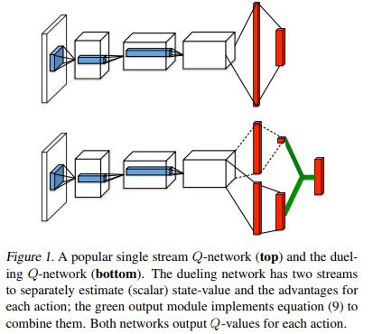
Dueling网络结构通过一个共享的深度神经网络表示了A: 状态值函数$V(s)$和B: Advantage函数 $A(s,a)$,该共享网络的输出将A与B网络的输出结合产生Q(s,a)值。
Advantage函数的定义为:
$$A^\pi (s, a) = Q^\pi (s, a) - V^\pi (s)$$
值函数$V(s)$表示状态s有多好,而Q(s,a)函数表示在状态s执行动作a有多好。通过上面的式子,可以得到:
$$ Q(s, a; \theta, \alpha, \beta) = V (s; \theta, \beta) + A(s, a; \theta, \alpha) $$
其中$\theta$代表前面的卷积神经网路参数, $\alpha$代表后面值函数$V(s)$的神经网络参数,$\beta$代表后面$Q(s,a)$函数的神经网络参数。
上面的式子存在不可辩问题,即已知$Q(s,a)$,$V(s)$和$A(s,a)$有无穷的组合,无法确定它们各自的值。为了解决该问题,可以强制让Advantage函数的网络在状态$s$下选择的动作$a$对应的advantage值C为0,即将Advantage的值都减去C,该方法保证可以通过$Q$将$V$和$A$恢复出来,公式如下:
$$ Q(s, a; \theta, \alpha, \beta) = V (s; \theta, \beta) + \big( A(s, a; \theta, \alpha) - \max_{a\prime \in |\mathcal{A}|} A(s, a\prime; \theta, \alpha) \big) $$
但是可以看出,上面的式子中Advantage函数需要拟合当任意的最优动作改变时对应的Advantage值,这会造成训练过程的不稳定,因此,改进方法是利用$A(s,a)$的平均值代替求最大值的操作,该方法的潜在意思是:相比于一直学习拟合最大的动作值对应的Advantage值,只需要拟合平均的动作值对应的Advantage值就好,公式如下:
$$ Q(s, a; \theta, \alpha, \beta) = V (s; \theta, \beta) + \big( A(s, a; \theta, \alpha) - \frac{1}{|\mathcal{A}|} \sum_{a\prime} A(s, a\prime; \theta, \alpha) \big) $$
代码实现细节
class Network(nn.Module):
    def __init__(self, in_dim: int, out_dim: int):
        """Initialization."""
        super(Network, self).__init__()

        # set common feature layer
        self.feature_layer = nn.Sequential(
            nn.Linear(in_dim, 128),
            nn.ReLU(),
        )

        # set advantage layer
        self.advantage_layer = nn.Sequential(
            nn.Linear(128, 128),
            nn.ReLU(),
            nn.Linear(128, out_dim),
        )

        # set value layer
        self.value_layer = nn.Sequential(
            nn.Linear(128, 128),
            nn.ReLU(),
            nn.Linear(128, 1),
        )

    def forward(self, x: torch.Tensor) -> torch.Tensor:
        """Forward method implementation."""
        feature = self.feature_layer(x)

        value = self.value_layer(feature)
        advantage = self.advantage_layer(feature)

        q = value + advantage - advantage.mean(dim=-1, keepdim=True)

        return q
Noisy Networks for Exploration
NoisyNet是一种探索方法,可以通过学习网络权重的扰动来促进策略的探索,主要认为对权重向量的微小更改会造成多个时间步中引发一致且可能非常复杂的状态相关的策略更改。
对于一个输入为p维,输出为q维的的线性神经元来说:
$$ y = wx + b $$
其中$x \in \mathbb{R}^p$是神经元输入, $w \in \mathbb{R}^{q \times p}$, $b \in \mathbb{R}$是神经元输出。
对应的Noisy 线性层为:
$$ y = (\mu^w + \sigma^w \odot \epsilon^w) x + \mu^b + \sigma^b \odot \epsilon^b $$
其中$\mu^w \in \mathbb{R}^{q \times p}, \mu^b \in \mathbb{R}^q, \sigma^w \in \mathbb{R}^{q \times p}$和$\sigma^b \in \mathbb{R}^q$ 是可学习的参数, $\epsilon^w \in \mathbb{R}^{q \times p}$和$\epsilon^b \in \mathbb{R}^q$是可以通过下面两种方式产生的随机噪声变量:
- Independent Gaussian Noise: 每一个添加给权重和偏置的随机噪声都是从单位高斯分布中采样和独立的,对于每一个线性神经元来说,将会有$pq+q$个噪声变量
- Factorised Gaussian Noise: 该方法对于运算来说非常高效。它通过生成2个随机高斯噪声向量$(p,q)$的外积来产生$pq+q$个随机噪声:
$$ \epsilon_{i,j}^w = f(\epsilon_i) f(\epsilon_j) $$
$$ \epsilon_{j}^b = f(\epsilon_i) $$
$$ f(x) = sgn(x) \sqrt{|x|} $$
代码实现细节
需要注意的是NoisyNet可以看做是$\epsilon-greedy$的一种,因此与$\epsilon$有关的代码都可以省去。
class NoisyLinear(nn.Module):
    """Noisy linear module for NoisyNet.

    Attributes:
        in_features (int): input size of linear module
        out_features (int): output size of linear module
        std_init (float): initial std value
        weight_mu (nn.Parameter): mean value weight parameter
        weight_sigma (nn.Parameter): std value weight parameter
        bias_mu (nn.Parameter): mean value bias parameter
        bias_sigma (nn.Parameter): std value bias parameter

    """
    def __init__(self,
                 in_features: int,
                 out_features: int,
                 std_init: float = 0.5):
        """Initialization."""
        super(NoisyLinear, self).__init__()

        self.in_features = in_features
        self.out_features = out_features
        self.std_init = std_init

        self.weight_mu = nn.Parameter(torch.Tensor(out_features, in_features))
        self.weight_sigma = nn.Parameter(
            torch.Tensor(out_features, in_features))
        self.register_buffer("weight_epsilon",
                             torch.Tensor(out_features, in_features))

        self.bias_mu = nn.Parameter(torch.Tensor(out_features))
        self.bias_sigma = nn.Parameter(torch.Tensor(out_features))
        self.register_buffer("bias_epsilon", torch.Tensor(out_features))

        self.reset_parameters()
        self.reset_noise()

    def reset_parameters(self):
        """Reset trainable network parameters (factorized gaussian noise)."""
        mu_range = 1 / math.sqrt(self.in_features)
        self.weight_mu.data.uniform_(-mu_range, mu_range)
        self.weight_sigma.data.fill_(self.std_init /
                                     math.sqrt(self.in_features))
        self.bias_mu.data.uniform_(-mu_range, mu_range)
        self.bias_sigma.data.fill_(self.std_init /
                                   math.sqrt(self.out_features))

    def reset_noise(self):
        """Make new noise."""
        epsilon_in = self.scale_noise(self.in_features)
        epsilon_out = self.scale_noise(self.out_features)

        # outer product
        self.weight_epsilon.copy_(epsilon_out.ger(epsilon_in))
        self.bias_epsilon.copy_(epsilon_out)

    def forward(self, x: torch.Tensor) -> torch.Tensor:
        """Forward method implementation.

        We don't use separate statements on training / evaluating mode.
        It doesn't show remarkable difference of performance.
        """
        return F.linear(
            x,
            self.weight_mu + self.weight_sigma * self.weight_epsilon,
            self.bias_mu + self.bias_sigma * self.bias_epsilon,
        )

    # 类的静态方法,跟普通函数没什么区别,与类和实例都没有所谓的绑定关系
    @staticmethod
    def scale_noise(size: int) -> torch.Tensor:
        """Set scale to make noise (factorized gaussian noise)."""
        x = torch.FloatTensor(np.random.normal(loc=0.0, scale=1.0, size=size))
        return x.sign().mul(x.abs().sqrt())
Categorical DQN
在Categorical DQN论文中,作者认为DQN的训练目标是学习奖惩值的分布而不是某个状态下的奖惩值期望,核心思想是奖惩值的分布满足一个贝尔曼方程的变体,即在$S_t$状态下选择动作$A_t$,在最优策略的情况下,奖惩值的回报应该与在$S_{t+1}$的状态下,根据最优策略选择的$A_{t+1}$后产生的奖惩值分布有关系,即可根据折扣因子将其收缩至0,并通过奖惩(或者随机情况下的奖惩值分布)进行偏移。他们提出利用投射到一个离散支持向量$z$上的概率质量来建模奖惩值的分布。离散支持向量$z$具有$N_{atoms} \in \mathbb{N}^+$ 个原子, 其中$z_i = V_{min} + (i-1) \frac{V_{max} - V_{min}}{N-1}$, $i \in {1, …, N_{atoms}}$。
以概率分布的角度的Q-learning变体是通过对目标分布建立一个新的支持向量,然后最小化当前分布$d_t$和目标分布$d_t\prime$之间的$KL(Kullbeck-Leibler)散度来进行训练。
$$ d_t\prime = (R_{t+1} + \gamma_{t+1} z, p_hat{{\theta}} (S_{t+1}, \hat{a}^*_{t+1})) $$
最小化目标:
$$ D_{KL} (\phi_z d_t\prime | d_t) $$
其中$\phi_z$ 是一个目标分布在固定向量空间$z$上的一个L2投影, $\hat{a}^*_{t+1} = \arg\max_{a} q_{\hat{\theta}} (S_{t+1}, a)$是在状态$S_{t+1}$下对应平均动作值函数$q_{\hat{\theta}} (S_{t+1}, a) = z^{T}p_{\theta}(S_{t+1}, a)$的最优动作。
代码实现细节
通过神经网络来表示一个参数化的分布,在DQN中,输出的大小变成了atom_size * out_dim,然后对每一个输出的动作值都进行softmax操作,这样确保了标准化不同动作值之间的差异。
通过每一个动作的Softmax分布于支持向量的内积操作来估计$Q(s_t, a_t)的值,其中支持向量为:
$$ {z_i = V_{min} + i\Delta z: 0 \le i < N}, \Delta z = \frac{V_{max} - V_{min}}{N-1} $$
$$ Q(s_t, a_t) = \sum_i z_i p_i(s_t, a_t) $$
其中 $p_i$ 是 $z_i$ 的概率分布,即Softmax函数的输出。
class Network(nn.Module):
    def __init__(self, in_dim: int, out_dim: int, atom_size: int,
                 support: torch.Tensor):
        """Initialization."""
        super(Network, self).__init__()

        self.support = support
        self.out_dim = out_dim
        self.atom_size = atom_size

        self.layers = nn.Sequential(nn.Linear(in_dim, 128), nn.ReLU(),
                                    nn.Linear(128, 128), nn.ReLU(),
                                    nn.Linear(128, out_dim * atom_size))

    def forward(self, x: torch.Tensor) -> torch.Tensor:
        """Forward method implementation."""
        dist = self.dist(x)
        q = torch.sum(dist * self.support, dim=2)

        return q

    def dist(self, x: torch.Tensor) -> torch.Tensor:
        """Get distribution for atoms."""
        q_atoms = self.layers(x).view(-1, self.out_dim, self.atom_size)
        dist = F.softmax(q_atoms, dim=2)

        return dist
N-Step Learning
Q-learning会利用一个单一的奖惩值和下一个状态下最优动作的Q值来进行自举(Bootstrap),该方法只能利用下一个时刻的信息,改进思路是向前多看几步,利用接下来的N步信息,这就是在状态$S_t$下的Truncated N-Step Return,定义为:
$$ R^{(n)}_t = \sum_{k=0}^{n-1} \gamma_t^{(k)} R_{t+k+1} $$
DQN的变体N-Step Learning的目标是通过最小化下面的损失函数:
$$ (R^{(n)}_t + \gamma^{(n)}_t \max_{a \prime} q_{\theta}^{-} (S_{t+n}, a \prime) - q_{\theta} (S_t, A_t))^2 $$
利用调整后的N-Step Learning通常会加速智能体的训练过程。
代码实现细节
这里和DQN不同的一点是利用deque来实现经验回放池:
class ReplayBuffer:
    """A simple numpy replay buffer."""

    def __init__(
            self,
            obs_dim: int,
            size: int,
            batch_size: int = 32,
            n_step: int = 3,
            gamma: float = 0.99,
    ):
        self.obs_buf = np.zeros([size, obs_dim], dtype=np.float32)
        self.next_obs_buf = np.zeros([size, obs_dim], dtype=np.float32)
        self.acts_buf = np.zeros(size, dtype=np.float32)
        self.rews_buf = np.zeros(size, dtype=np.float32)
        self.done_buf = np.zeros(size, dtype=np.float32)
        self.max_size, self.batch_size = size, batch_size
        self.ptr, self.size, = 0, 0

        # for N-step Learning
        self.n_step_buffer = deque(max_len=n_step)
        self.n_step = n_step
        self.gamma = gamma

    def store(self, obs: np.ndarray, act: np.ndarray, rew: float,
              next_obs: np.ndarray, done: bool
              ) -> Tuple[np.ndarray, np.ndarray, float, np.ndarray, bool]:
        transition = (obs, act, rew, next_obs, done)
        self.n_step_buffer.append(transition)

        # single step transition is not ready
        if len(self.n_step_buffer) < self.n_step:
            return ()

        # make a n-step transition
        rew, next_obs, done = self._get_n_step_info(self.n_step_buffer,
                                                    self.gamma)
        obs, act = self.n_step_buffer[0][:2]

        self.obs_buf[self.ptr] = obs
        self.next_obs_buf[self.ptr] = next_obs
        self.acts_buf[self.ptr] = act
        self.rews_buf[self.ptr] = rew
        self.done_buf[self.ptr] = done
        self.ptr = (self.ptr + 1) % self.max_size
        self.size = min(self.size + 1, self.max_size)

        return self.n_step_buffer[0]

    def sample_batch(self) -> Dict[str, np.ndarray]:
        indices = np.random.choice(self.size,
                                   size=self.batch_size,
                                   replace=False)

        return dict(
            obs=self.obs_buf[indices],
            next_obs=self.next_obs_buf[indices],
            acts=self.acts_buf[indices],
            rews=self.rews_buf[indices],
            done=self.done_buf[indices],
            # for N-step Learning
            indices=indices,
        )

    def sample_batch_from_idxs(self,
                               indices: np.ndarray) -> Dict[str, np.ndarray]:
        # for N-step Learning
        return dict(
            obs=self.obs_buf[indices],
            next_obs=self.next_obs_buf[indices],
            acts=self.acts_buf[indices],
            rews=self.rews_buf[indices],
            done=self.done_buf[indices],
        )

    def _get_n_step_info(self, n_step_buffer: Deque,
                         gamma: float) -> Tuple[np.int64, np.ndarray, bool]:
        """Return n step rew, next_obs, and done."""
        # info of the last transition
        rew, next_obs, done = n_step_buffer[-1][-3:]

        for transition in reversed(list(n_step_buffer)[:-1]):
            r, n_o, d = transition[-3:]

            rew = r + gamma * rew * (1 - d)
            next_obs, done = (n_o, d) if d else (next_obs, done)

        return rew, next_obs, done

    def __len__(self) -> int:
        return self.size
Reference
- Human-level Control through Deep Reinforcement Learning
- Deep Reinforcement Learning with Double Q-learning
- Prioritized Experience Replay
- Dueling Network Architectures for Deep Reinforcement Learning
- Noisy Networks for Exploration
- A Distributional Perspective on Reinforcement Learning
- Learning to Predict by the Methods of Temporal Differences
- Rainbow is All You Need
Note: Cover Picture